How To Plot N-simple Moving Average Fir Filter In Matlab

The moving average filter is a simple Depression Pass FIR (Finite Impulse Response) filter commonly used for smoothing an array of sampled data/signal. It takes $L$ samples of input at a time and takes the boilerplate of those $L$ -samples and produces a single output point. It is a very elementary LPF (Low Pass Filter) structure that comes handy for scientists and engineers to filter unwanted noisy component from the intended information.

As the filter length increases (the parameter $L$ ) the smoothness of the output increases, whereas the abrupt transitions in the data are made increasingly blunt. This implies that this filter has first-class time domain response but a poor frequency response.

The MA filter performs three important functions:

ane) It takes $L$ input points, computes the average of those $L$ -points and produces a unmarried output point
two) Due to the computation/calculations involved, the filter introduces a definite amount of delay
3) The filter acts as a Low Laissez passer Filter (with poor frequency domain response and a good time domain response).

Implementation

The difference equation for a $L$ -point discrete-time moving average filter with input represented by the vector $\mathbf{x}$ and the averaged output vector $\mathbf{y}$ , is

\[y[n] = \displaystyle{\frac{1}{L} \sum_{k=0}^{L-ane}ten[n-k]} \quad\quad (one) \]

For example, a $5$ -betoken Moving Average FIR filter takes the electric current and previous four samples of input and calculates the boilerplate. This operation is represented as shown in the Effigy 1 with the following departure equation for the input output human relationship in detached-fourth dimension.

\[\brainstorm{aligned} y[n] &= \displaystyle{\frac{1}{5} \left(ten[n] + ten[n-1] + 10[n-2] + x[n-3] + x[n-4] \right) } \\ &= 0.2 \left(10[north] + x[n-ane] + x[n-2] + 10[n-iii] + x[n-iv] \right) \cease{aligned} \quad\quad (two) \]

Effigy 1: Detached-fourth dimension 5-point Moving Boilerplate FIR filter

The unit delay shown in Effigy 1 is realized past either of the ii options:

Z-Transform and Transfer function

In bespeak processing, delaying a signal $x[n]$ by $k$ sample catamenia (unit filibuster) is equivalent to multiplying the Z-transform $X[z]$ by $z^{-k}$ . Past applying this idea, nosotros can find the Z-transform of the $5$ -indicate moving average filter in equation (2) as

\[ \begin{aligned} y[northward] &= 0.2 \left(x[n] + ten[n-1] + 10[n-2] + ten[northward-3] + x[north-4] \right) \\ Y[z] &= 0.two \left(z^0 + z^{-ane} + z^{-2} + z^{-three} + z^{-4} \right) X[z] \\ Y[z] &= 0.2 \left(1 + z^{-1} + z^{-two} + z^{-iii} + z^{-iv} \right) X[z] \quad\quad (three) \end{aligned}\]

Similarly, the Z-transform of the generic $L$ -sample Moving Average filter of equation (1) is

\[x Y(z) = \left(\displaystyle{\frac{1}{L} \sum_{chiliad=0}^{L-1} z^{-1000}} \correct) Ten(z) \quad\quad (4) \]

The transfer function describes the input-output relationship of the arrangement and for the $L$ -betoken Moving Average filter, the transfer function is given by

\[H(z) = \displaystyle{\frac{Y(z)}{X(z)}} =\displaystyle{\frac{1}{L} \sum_{thou=0}^{L-1} z^{-one thousand}} \quad\quad (5)\]

Simulating the filter in Matlab and Python

In Matlab, we tin can employ the filter function or conv (convolution) to implement the moving boilerplate FIR filter.

In general, the Z-transform $Y(z)$ of a discrete-fourth dimension filter's output $y(n)$ is related to the Z-transform $X(z)$ of the input $x(n)$ by

\[H(z) = \displaystyle{\frac{Y(z)}{X(z)}} = \displaystyle{\frac{b_0 + b_1 z^{-1} + b_2 z^{-2} + \cdots + b_n z^{-n}}{a_0 + a_1 z^{-1} + a_2 z^{-2} + \cdots + a_m z^{-m}}} \quad\quad (6) \]

where, $\{b_i\}$ and $\{a_i\}$ are the filter coefficients and the club of the filter is the maximum of $n$ and $m$

For implementing equation (6) using the filter function, the Matlab function is called every bit

B = [b_0, b_1, b_2, ..., b_n] %numerator coefficients A = [a_0, a_1, a_2, ..., a_m] %denominator coefficients y = filter(B,A,10) %filter input ten and get result in y

We can note from the difference equation and transfer role of the $L$ -signal moving average filter, that post-obit values for the numerator coefficients $\{b_i\}$ and denominator coefficients $\{a_i\}$ .

\[\begin{aligned} \{b_i\} &= \{1/Fifty, 1/L, …., 1/L\} &,i=0,1,\cdots,50-1 \\ \{a_i\} &= {ane} &,i=0 \terminate{aligned} \quad\quad (7)\]

Therefore, the $5$ -betoken moving average filter can be coded as

B = [0.2, 0.2, 0.two, 0.2, 0.2] %numerator coefficients A = [one] %denominator coefficients y = filter(B,A,x) %filter input ten and get effect in y

The numerator coefficients for the moving average filter tin be conveniently expressed in short notion as shown beneath

          L = five B = ones(one,Fifty)/L %numerator coefficients A = [1] %denominator coefficients ten = rand(1,x) %random samples for x y = filter(B,A,x) %filter input ten and get result in y

When using conv function to implement the moving average filter, the following lawmaking tin can be used

L = 5; x = rand(1,10) %random samples for x; y = conv(x,ones(ane,L)/50)

At that place exists a difference between using conv function and filter role for implementing an FIR filter. The conv role gives the result of complete convolution and the length of the result is length(10)+ L -ane . Whereas, the filter function gives the output that is of same length equally that of the input $x$ .

In python, the filtering operation can exist performed using the lfilter and convolve functions available in the scipy signal processing package. The equivalent python code is shown below.

import numpy every bit np from scipy import point L=5 #L-indicate filter b = (np.ones(L))/50 #numerator co-effs of filter transfer function a = np.ones(one)  #denominator co-effs of filter transfer part 10 = np.random.randn(ten) #10 random samples for 10 y = signal.convolve(x,b) #filter output using convolution  y = betoken.lfilter(b,a,x) #filter output using lfilter function

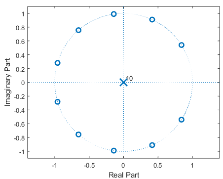
Pole-nada plot and frequency response

A pole-zero plot for a filter transfer role $H(z)$ , displays the pole and zero locations in the z-plane. In the pole-zero plot, the zeros occur at locations (frequencies) where $H(z) \rightarrow 0$ and the poles occur at locations (frequencies) where $H(z) \rightarrow \infty$ . Equivalently, zeros occurs at frequencies for which the numerator of the transfer function in equation vi becomes zero and the poles occurs at frequencies for which the denominator of the transfer role becomes nothing.

In a pole-zero plot, the locations of the poles are usually marked by cross ( $\times$ ) and the zeros are marked as circles ( $\circ$ ). The poles and zeros of a transfer function effectively define the arrangement response and determines the stability and operation of the filtering arrangement.

In Matlab, the pole-nil plot and the frequency response of the $L$ -betoken moving average tin be obtained every bit follows.

Fifty=11 zplane([ones(one,Fifty)]/50,1); %pole-zero plot due west = -pi:(pi/100):pi; %to plot frequency response freqz([ones(i,Fifty)]/Fifty,1,w); %plot magnitude and phase response

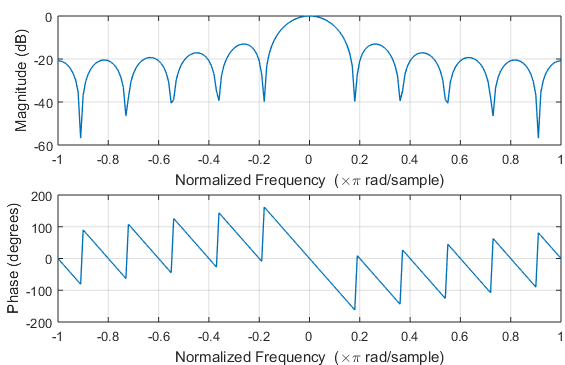
Figure 2: Pole-Naught plot for 50=xi-bespeak Moving Average filter

Effigy 3: Magnitude and phase response of L=eleven-point Moving Average filter

The magnitude and stage frequency responses can be coded in Python equally follows

[updated] See my Google colab for full Python code

import numpy equally np from scipy import point import matplotlib.pyplot as plt  L=11 #Fifty-point filter b = (np.ones(L))/50 #numerator co-effs of filter transfer office a = np.ones(1)  #denominator co-effs of filter transfer function  w, h = bespeak.freqz(b,a) plt.subplot(2, 1, one) plt.plot(w, 20 * np.log10(abs(h))) plt.ylabel('Magnitude [dB]') plt.xlabel('Frequency [rad/sample]')  plt.subplot(two, 1, ii) angles = np.unwrap(np.angle(h)) plt.plot(westward, angles) plt.ylabel('Bending (radians)') plt.xlabel('Frequency [rad/sample]') plt.show()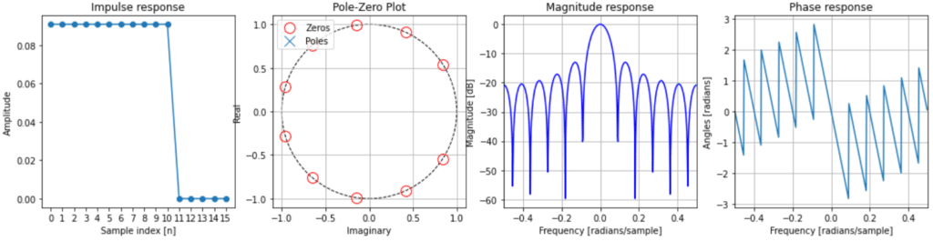

Impulse response, Pole-zero plot, magnitude and phase response of L=11 moving average filter — Figure 4: Impulse response, Pole-zero plot, magnitude and phase response of L=11 moving boilerplate filter

Case report:

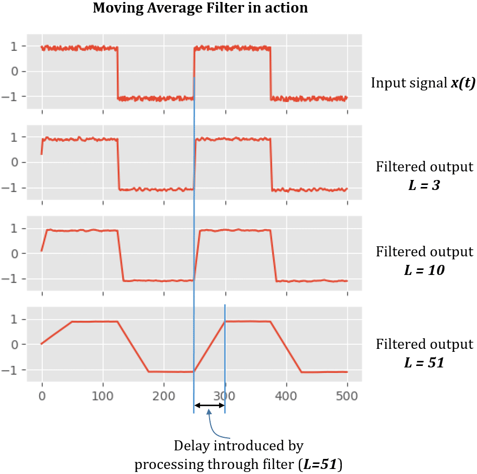
Following figures depict the time domain & frequency domain responses of a $L$ -bespeak Moving Boilerplate filter. A noisy foursquare wave signal is driven through the filter and the time domain response is obtained.

Processing a signal through Moving average filter of various lengths — *Effigy 5: Processing a bespeak through Moving average filter of various lengths*

On the first plot, nosotros have the noisy square moving ridge point that is going into the moving average filter. The input is noisy and our objective is to reduce the dissonance equally much every bit possible. The next effigy is the output response of a 3-indicate Moving Average filter. It can be deduced from the figure that the 3-bespeak Moving Average filter has non done much in filtering out the noise. We increment the filter taps to 10-points and we tin can come across that the racket in the output has reduced a lot, which is depicted in next figure.

With L=51 tap filter, though the racket is nigh zero, the transitions are blunted out drastically (detect the gradient on the either side of the point and compare them with the platonic brick wall transitions in the input indicate).

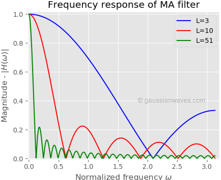
*Effigy 6: Frequency response of moving average filters of various lengths*

From the frequency response of lower society filters ( L=3, Fifty=10 ), it can exist asserted that the roll-off is very boring and the stop ring attenuation is not practiced. Given this stop band attenuation, clearly, the moving average filter cannot divide one band of frequencies from another. As we increment the filter order to 51, the transitions are not preserved in time domain. Expert performance in the time domain results in poor performance in the frequency domain, and vice versa. Compromise need for optimal filter design.

Rate this article: Poor Below average Average Good Excellent (46 votes, average: iv.41 out of v)

References:

[1] Filtering – OpenCourseWare – MIT.↗
[ii] HC Chen et al.,"Moving Average Filter with its application to QRS detection",IEEE Computers in Cardiology, 2003.↗

Books by the writer